RNA-Seq oriented questions

Why the --seqbias in Salmon?

From Salmon documentation, we can read that Salmon is able to learn and correct sequence-specific bias. It models the (not-so-)random hexamer printing bias and tries to correct it. By default, Salmon learns the sequence-specific bias parameters using 1,000,000 reads from the beginning of the input. Salmon uses a variable-length Markov Model (VLMM) to model the sequence specific biases at both the 5’ and 3’ end of sequenced fragments. This methodology generally follows that of Roberts et al., though some details of the VLMM differ.

This options keeps us from trimming the ~13 first nucleotides in the beginning of every reads in our RNA-Seq data. Usually, these nucleotides present a lot of errors and/or enrichment (the preferential sequencing of fragments starting with certain nucleotide motifs).

What is bootstrapping?

From Salmon documentation, we can read that Salmon is able to perform bootstraps. We strongly recommend to perform at least 35 bootstraps rounds in order to have a correct estimation of the technical variance within each of your samples.

Bootstrapped abundance estimates are done by re-sampling (with replacement) from the counts assigned to the fragment equivalence classes, and then re-running the optimization procedure, either the EM or VBEM (see below for more information), for each such sample. The values of these different bootstraps allows us to assess technical variance in the main abundance estimates we produce. Such estimates can be useful for downstream (e.g. differential expression) tools that can make use of such uncertainty estimates. The more samples computed, the better the estimates of variance, but the more computation (and time) required.

Why the –gcbias in Salmon ?

From Salmon documentation, we can read that Salmon is able to learn and correct fragment-level GC biases in the input data. Specifically, this model will attempt to correct for biases in how likely a sequence is to be observed based on its internal GC content.

A strong GC bias is often a sign of an enrichment in a given sequence, a contamination or a sequencing error. GC Bias correction does not impair quantification for samples without GC bias. For samples with moderate to high GC bias, correction for this bias at the fragment level has been shown to reduce isoform quantification errors: Patro et al., and Love et al..

This bias is distinct from the primer biases previously described. Though these biases are distinct, they are not completely independent.

How was the kmer length chosen in Salmon?

A k-mer is a word of length “k”. A Dimer is a k-mer of length 2. A Pentamer is a k-mer of length 5, etc. To be specific of a region, due to the length of the human genome, we strongly recommend a value above 27 (usually, the default value of 31 is enough, see Srivastava et al.).

However, shorter reads are discarded. This means that any sequence of length below 31 will not appear here, or will present potential analysis bias.

How was the sequencing library parameter chosen?

From Salmon documentation, we can read that all theoretical positions of reads are taken into account by Salmon.

There are numerous library preparation protocols for RNA-seq that result in sequencing reads with different characteristics. For example, reads can be single end (only one side of a fragment is recorded as a read) or paired-end (reads are generated from both ends of a fragment). Further, the sequencing reads themselves may be un-stranded or strand-specific. Finally, paired-end protocols will have a specified relative orientation.

• I = inward

• O = outward

• M = matching

• S = stranded

• U = un-stranded

• F = read 1 (or single-end read) comes from the forward strand

• R = read 1 (or single-end read) comes from the reverse strand

• A = Automatic detection

What is mapping validation in Salmon ?

From Salmon documentation, we can read that Salmon can perform mapping validation:

One potential artifact that may arise from alignment-free mapping techniques is spurious mappings. These may either be reads that do not arise from some target being quantified, but nonetheless exhibit some match against them (e.g. contaminants) or, more commonly, mapping a read to a larger set of quantification targets than would be supported by an optimal or near-optimal alignment.

Salmon will run an extension alignment dynamic program on the quasi-mappings it produces. Moreover, Salmon makes use of an intelligent alignment cache to avoid re-computing alignment scores against redundant transcript sequences (e.g. when a read maps to the same exon in multiple different transcripts).

Quality trimming is more important before processing reads using this option.

What is quasi-mapping?

From Salmon documentation, we can read that:

One of the novel and innovative features of Salmon is its ability to accurately quantify transcripts using quasi-mappings. Quasi-mappings are mappings of reads to transcript positions that are computed without performing a base-to-base alignment of the read to the transcript. Quasi-mapping is typically much faster to compute than traditional (or full) alignments, and can sometimes provide superior accuracy by being more robust to errors in the read or genomic variation from the reference sequence.

The quasi-mapping was introduced in the work of Srivastava et al., and Bray et al..

Remember that reads are broken into k-mers (here, k-mers of length 31). These k-mers are stored in a large and effective associative table, in which maximum mapable prefix are computed for each k-mer. Then, each probable position if compared in order to find a longest common prefix.

In short: reads are never mapped, but k-mer built from the reads are searched in a large associative table.

What is the Expected-Maximization Algorithm?

Expected maximization algorithm is a method used to estimate the transcript abundances based on previously observed data within the sample. The main idea of this approach stands in two points:

> For each read, given a range of positions where this read comes from, guess the probability this read comes from a given position Knowing previous assignations, adjust the guessing-pattern

It has been shown by Capellini et al., then by Dempster et al., that EM algorithm converges when steps one and two are repeatedly applied one after each other.

What is Variational Bayesian Expected-Maximisation Algorithm?

From Salmon documentation, we can find the following explanation about differences between EM algorithm, and the VBEM:

The details of the VBEM algorithm can be found in the article of Patro et al. While both the standard EM and the VBEM produce accurate abundance estimates, there are some trade-offs between the approaches. Specifically, the sparsity of the VBEM algorithm depends on the prior that is chosen. When the prior is small, the VBEM tends to produce a sparser solution than the EM algorithm, while when the prior is relatively larger, it tends to estimate more non-zero abundances than the EM algorithm. It is an active research effort to analyze and understand all the tradeoffs between these different optimization approaches. Also, the VBEM tends to converge after fewer iterations, so it may result in a shorter runtime; especially if you are computing many bootstrap samples.

What is the argument –gencode in Salmon?

This is a purely aesthetic option. Usually a genic object is identified with either: a gene name from HUGO (i.e. PTEN, BRCA1, …), or from ENSEMBL (i.e. ENSG00000171862, ENSG00000012048, …), etc. In its transcript genome sequences, Gencode uses multiple identifiers and separates them with a pipe (|).

As this is very convenient to search for names, transcripts, and protein correspondence, this also breaks compatibility with downstream tools. Salmon automatically breaks Gencodes names into a unique Ensembl identifier.

What are TPM? Why not use Raw couts, FPKM or RPM ?

TPM, FPKM, RPKM, and RPM are metrics which attempt to normalize the raw read count into a score. A very good youtube video explains it and the following text repeats the video’s message:

In order to compare two values, the have to refer to the same scale. It is the very same process when you try to compare to academic averages: (12/20 and 3/5 are equal grades).

Here, in RNA-Seq, we have similar issues. The main issues are:

1. There is not the very same amount of biological material in all sequenced samples

2. Longer genes take longer time to be replicated, they will have fewer reads

RPM (Reads per Milion), only solved the first issue described above. To compute your RPM, you have to:

1. Count up the total reads in a sample and divide that number by 1,000,000 – this is our “per million” scaling factor.

2. Divide the read counts by the “per million” scaling factor. This normalizes for sequencing depth, giving you reads per million (RPM)

This metric has quickly been deprecated, yet many teams around the world still uses it, ignoring elementary PCR bias.

The idea was then to correct the read count by the gene length. There, the RPKM (Read Per Kilobase per Million) was born. Here’s how you do it for RPKM:

1. Count up the total reads in a sample and divide that number by 1,000,000 – this is our “per million” scaling factor.

2. Divide the read counts by the “per million” scaling factor. This normalizes for sequencing depth, giving you reads per million (RPM)

3. Divide the RPM values by the length of the gene, in kilobases. This gives you RPKM.

Applied to Paired-end sequencing, this normalisation relies not on read-counts anymore, but on a pair-of-read counts. A pair of reads is called a fragment. There, the FPKM (Fragment Per Kilobase per Million) was born.

With RPKM or FPKM, the sum of normalized reads in each sample can be different. It means FPKM and RPKM does not solve the problem. They just reduce it.

Finally, TPM (Transcript Per Million), just switches two steps of the FPKM method, but solves the two issues presented at the beginning of this section. Here’s how you calculate TPM:

1. Divide the read counts by the length of each gene in kilobases. This gives you reads per kilobase (RPK).

2. Count up all the RPK values in a sample and divide this number by 1,000,000. This is your “per million” scaling factor.

3. Divide the RPK values by the “per million” scaling factor. This gives you TPM.

Kanitz et al., and Dillies et al. compares various methods of normalization including RPKM and TPM. If you persist in willing to use FPKM over TPM, you are doing things wrong when you compare two samples. Yet, you can use FPKM to compare two genes in one sample.

P-Value, Adjusted P-Value or Q-Value

P-Values and Q-Values are metrics used to rank observation from 0 (effective difference) to 1 (purely random observation). A Q-Value is a P-Value adjusted using an optimized FDR (False Discovery Rate) approach.

A P-Value of 0.05 implies that 5% of all tests will result in false positives. A Q-Value of 0.05 implies that 5% of significant tests will result in false positives. The second includes a lot less of false positive.

Here is an example from nonlinear.com:

Let us imagine an experiment with 3516 biochemical compound. If we take a compound which has a p-value of 0.0101 and a q-value of 0.0172.

Recall that a p-value of 0.0101 implies a 1.01% chance of false positives, and so with 3516 compounds, we expect about 36 false positives, i.e. 3516 × 0.0101 = 35.51. In this experiment, there are 800 compounds with a value of 0.0101 or less, and so 36 of these will be false positives.

On the other hand, the q-value is 0.0172, which means we should expect 1.72% of all the compounds with q-value less than this to be false positives. This is a much better situation. We know that 800 compounds have a q-value of 0.0172 or less and so we should expect 800 × 0.0172 = 13.76 false positives rather than the predicted 36.

Always consider Q-Values or Adjusted P-Values rather than (raw) P-Values.

Fold change and significance

The Fold Change is a simple ratio over two observations:

\(FC = \frac{mean(Expression gene A, condition 1)}{mean(Expression gene A, condition 2)}\)

We use a Log2(FC) for plotting convenience.

By itself, a Fold Change does not lead to any conclusion: a high fold change may be due to anything from the initial hypothesis to any other kind of external factor. That’s why we use DESeq2 to perform the differential expression analysis, rather than a simple ratio.

The point of DESeq2 is to conclude, with a P-Value, weather the expression variation seems to be related to our initial hypothesis or not.

Let us consider the following cases, which are classic misleading cases in which a high Fold Change is not related to our initial hypothesis.

Out layers

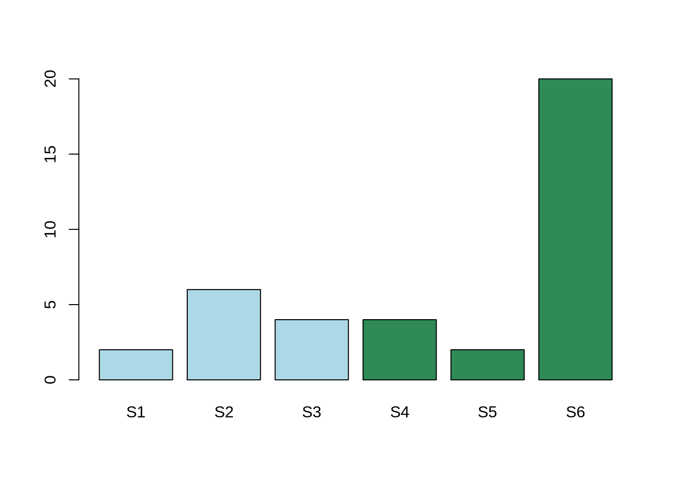
Here, the mean expression for the gene Gene1 for condition A is: 4. The mean expression for the gene Gene2 for condition B is: 8.6.

The mean expression in the two conditions are different, however, this difference is due to one single sample which is not behaving like the others.

In conclusion, there is indeed a variation. This variation is due to one sample, rather than one condition. In that case, the adjusted P-Value will be high and considered as non-significant. We are not interested in the variability on one sample. We are interested in the variability of one global condition.

Intra-class variability

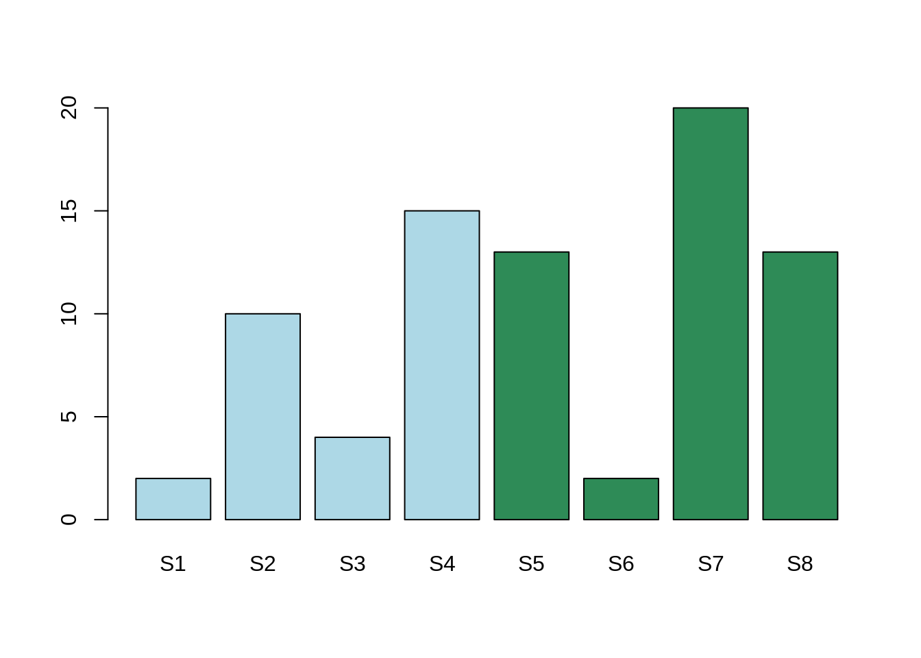
Here, the mean expression for the gene Gene1 for condition A is: 4. The mean expression for the gene Gene2 for condition B is: 8.6.

The mean expression in the two conditions are different, however, this difference is less than the expression variability within both Condition A and Condition B.

The differential expression is more likely to be between samples 1, 3, and 6 in one hand, and 2, 4, 5, 7 and 8 in the other hand.

In conclusion, there is indeed a variation. This variation seems not related to our hypothesis, rather than an unknown factor. This unknown factor is called “confounding factor”. In this case, the adjusted P-Value will be high and, therefore, non significant.

Simpson Paradox

In this case, we have nested conditions. Let’s imagine a tumor, which can be treated by either chemotherapy or surgery. We want to know which one perform better. For the last 1000 treated patients, you will find below the success rate of each of these methods:

Treatment	Nb. recoveries	Nb. failures	Recovery rate
Chemotherapy	761	239	76%
Surgery	658	342	66%

It seems clear that the chemotherapy performs better than surgery.

However, if you consider the tumor size, the numbers are the following:

Treatment	Tumor size	Nb. recoveries	Nb. failures	Recovery rate
Chemotherapy	> 2cm (large)	90	92	49%
Chemotherapy	< 2cm (small)	564	331	63%
Surgery	> 2cm (large)	94	11	90%
Surgery	< 2cm (small)	671	147	82%

Now, considering the tumor size, the surgery always perform better! You can check the numbers, both table talk about the very same numbers!

Taking the number in one table or the other changes the conclusion, how to decide ?! How can chemotherapy perform better while, taking into account the tumor size, surgery outperforms ? This is called the Simpson paradox.

There are two possible observations here:

• Smaller tumors have a higher recovery rate, which is not surprising.

• On large tumors, surgery is used more often than chemotherapy.

So, surgery performs better, however, it is used more often on difficult cases.

Here, “Treatment” is our factor of interest. “Tumor size” is a confounding factor. Surgery is used on larger tumors. The tumor size acts on both, cause and consequence in our analysis.

Conclusion:

If your bioinformatician chose to keep a given additional factor in your analysis, there is a reason. If a gene of interest appears while and only while this additional factor is (is is not) taken into account, you cannot chose the differential analysis you prefer in order to satisfy your initial hypothesis. You could fall under this kind of statistical traps. Your bioinformatician is here to help you!